Kalman Filter

The Kalman Filter is an algorithm that uses a series of measurements observed over time, containing statistical noise and other inaccuracies, and produces estimates of unknown variables. The filter is named after Rudolf E. Kálmán, who is one of the primary developers of its theory.

Assumptions and Model

The Kalman Filter assumes that the system is linear and that the current state can be described by a set of linear equations. The system model is described by the following equations:

$$ \mathbf{x}{k} = \mathbf{A}{k-1} \mathbf{x}{k-1} + \mathbf{B}{k-1} \mathbf{u}{k-1} + \mathbf{w}{k-1} $$

$$ \mathbf{z}{k} = \mathbf{H}{k} \mathbf{x}{k} + \mathbf{v}{k} $$

where:

• \( \mathbf{x}_{k} \) is the state vector at time \( k \)
• \( \mathbf{A}{k-1} \) is the state transition model which applies to the previous state \( \mathbf{x}{k-1} \)
• \( \mathbf{B}{k-1} \) is the control-input model which applies to the control vector \( \mathbf{u}{k-1} \)
• \( \mathbf{w}{k-1} \) is the process noise which is assumed to be drawn from a zero-mean multivariate normal distribution with covariance \( \mathbf{Q}{k-1} \)
• \( \mathbf{z}_{k} \) is the observation vector at time \( k \)
• \( \mathbf{H}_{k} \) is the observation model which maps the true state space into the observed space
• \( \mathbf{v}{k} \) is the observation noise which is assumed to be zero-mean Gaussian white noise with covariance \( \mathbf{R}{k} \)

Steps of the Kalman Filter

The Kalman Filter operates in two phases: the Prediction and the Update.

Prediction Phase

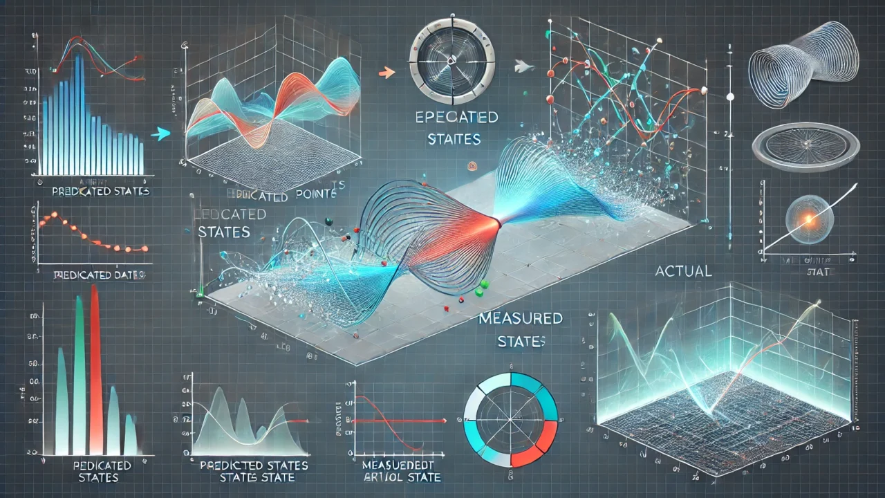
In the prediction phase, the filter produces estimates of the current state variables, along with their uncertainties. The prediction equations are:

1. Predicted state estimate:

$$ \mathbf{\hat{x}}{k|k-1} = \mathbf{A}{k-1} \mathbf{\hat{x}}{k-1|k-1} + \mathbf{B}{k-1} \mathbf{u}_{k-1} $$

2. Predicted estimate covariance:

$$ \mathbf{P}{k|k-1} = \mathbf{A}{k-1} \mathbf{P}{k-1|k-1} \mathbf{A}{k-1}^\top + \mathbf{Q}_{k-1} $$

Update Phase

In the update phase, the filter incorporates the new observation into the predicted state to refine the state estimate. The update equations are:

1. Innovation or measurement residual:

$$ \mathbf{y}{k} = \mathbf{z}{k} – \mathbf{H}{k} \mathbf{\hat{x}}{k|k-1} $$

2. Innovation covariance:

$$ \mathbf{S}{k} = \mathbf{H}{k} \mathbf{P}{k|k-1} \mathbf{H}{k}^\top + \mathbf{R}_{k} $$

3. Optimal Kalman gain:

$$ \mathbf{K}{k} = \mathbf{P}{k|k-1} \mathbf{H}{k}^\top \mathbf{S}{k}^{-1} $$

4. Updated state estimate:

$$ \mathbf{\hat{x}}{k|k} = \mathbf{\hat{x}}{k|k-1} + \mathbf{K}{k} \mathbf{y}{k} $$

5. Updated estimate covariance:

$$ \mathbf{P}{k|k} = ( \mathbf{I} – \mathbf{K}{k} \mathbf{H}{k} ) \mathbf{P}{k|k-1} $$

Detailed Proof

Prediction Equations

1. Predicted State Estimate:

Starting with the state equation:

$$ \mathbf{x}{k} = \mathbf{A}{k-1} \mathbf{x}{k-1} + \mathbf{B}{k-1} \mathbf{u}{k-1} + \mathbf{w}{k-1} $$

Taking the expectation:

$$ \mathbb{E}[\mathbf{x}{k}] = \mathbf{A}{k-1} \mathbb{E}[\mathbf{x}{k-1}] + \mathbf{B}{k-1} \mathbb{E}[\mathbf{u}_{k-1}] $$

Since \( \mathbf{w}_{k-1} \) is zero-mean:

$$ \mathbf{\hat{x}}{k|k-1} = \mathbf{A}{k-1} \mathbf{\hat{x}}{k-1|k-1} + \mathbf{B}{k-1} \mathbf{u}_{k-1} $$

2. Predicted Estimate Covariance:

The covariance of the predicted state estimate is:

$$ \mathbf{P}{k|k-1} = \mathbb{E}[(\mathbf{x}{k} – \mathbf{\hat{x}}{k|k-1})(\mathbf{x}{k} – \mathbf{\hat{x}}_{k|k-1})^\top] $$

Substituting

$$ \mathbf{x}{k} = \mathbf{A}{k-1} \mathbf{x}{k-1} + \mathbf{B}{k-1} \mathbf{u}{k-1} + \mathbf{w}{k-1} ) $$

$$ ( \mathbf{\hat{x}}{k|k-1} = \mathbf{A}{k-1} \mathbf{\hat{x}}{k-1|k-1} + \mathbf{B}{k-1} \mathbf{u}_{k-1} $$

$$ \mathbf{P}{k|k-1} = \mathbf{A}{k-1} \mathbf{P}{k-1|k-1} \mathbf{A}{k-1}^\top + \mathbf{Q}_{k-1} $$

Update Equations

1. Innovation:

$$ \mathbf{y}{k} = \mathbf{z}{k} – \mathbf{H}{k} \mathbf{\hat{x}}{k|k-1} $$

2. Innovation Covariance:

$$ \mathbf{S}{k} = \mathbf{H}{k} \mathbf{P}{k|k-1} \mathbf{H}{k}^\top + \mathbf{R}_{k} $$

3. Optimal Kalman Gain:

$$ \mathbf{K}{k} = \mathbf{P}{k|k-1} \mathbf{H}{k}^\top \mathbf{S}{k}^{-1} $$

4. Updated State Estimate:

$$ \mathbf{\hat{x}}{k|k} = \mathbf{\hat{x}}{k|k-1} + \mathbf{K}{k} \mathbf{y}{k} $$

5. Updated Estimate Covariance:

$$ \mathbf{P}{k|k} = ( \mathbf{I} – \mathbf{K}{k} \mathbf{H}{k} ) \mathbf{P}{k|k-1} $$

This completes the detailed explanation and proof of the Kalman Filter.