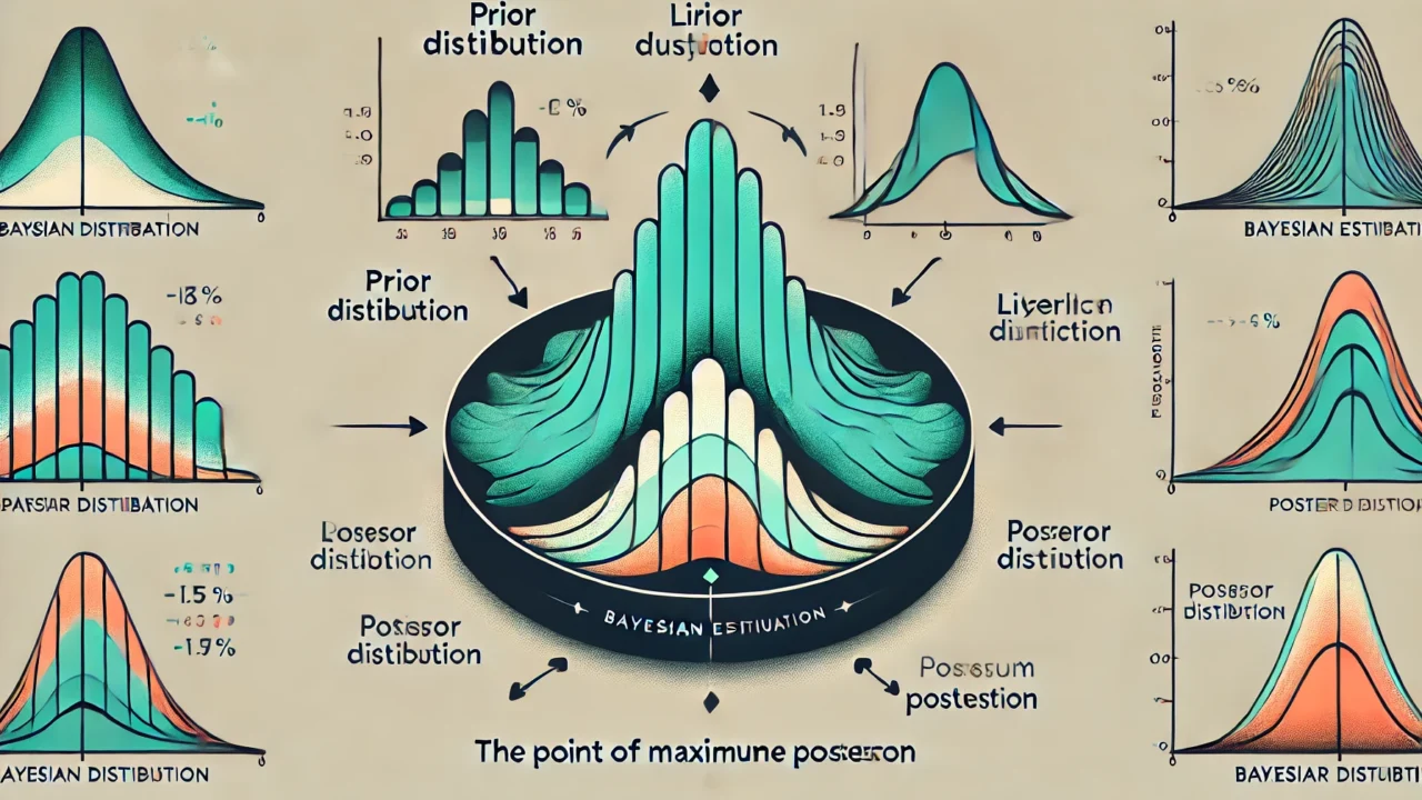
Bayesian estimation is a method in Bayesian statistics to estimate an unknown quantity based on prior information and observed data. The main goal is to update the prior belief about a parameter \( \theta \) given new data \( \mathbf{X} \). This is achieved through Bayes’ theorem.
Bayes’ Theorem
Bayes’ theorem relates the conditional and marginal probabilities of random events. For a parameter \( \theta \) and data \( \mathbf{X} \), it is given by:
$$ P(\theta \mid \mathbf{X}) = \frac{P(\mathbf{X} \mid \theta) P(\theta)}{P(\mathbf{X})} $$
Where:
\( P(\theta \mid \mathbf{X}) \) is the posterior probability of \( \theta \) given data \( \mathbf{X} \)
\( P(\mathbf{X} \mid \theta) \) is the likelihood of data \( \mathbf{X} \) given parameter \( \theta \)
\( P(\theta) \) is the prior probability of \( \theta \)
\( P(\mathbf{X}) \) is the marginal likelihood or evidence
Posterior Distribution
The posterior distribution \( P(\theta \mid \mathbf{X}) \) represents the updated belief about the parameter \( \theta \) after observing the data \( \mathbf{X} \). It is proportional to the product of the likelihood and the prior:
$$ P(\theta \mid \mathbf{X}) \propto P(\mathbf{X} \mid \theta) P(\theta) $$
Prior Distribution
The prior distribution \( P(\theta) \) reflects the initial belief about the parameter \( \theta \) before observing any data. It is based on previous knowledge or assumptions.
Likelihood
The likelihood function \( P(\mathbf{X} \mid \theta) \) describes the probability of the observed data \( \mathbf{X} \) given the parameter \( \theta \). It is a function of \( \theta \) with \( \mathbf{X} \) fixed.
Example
Suppose we have observed data \( \mathbf{X} = {x_1, x_2, \ldots, x_n} \) and we assume a Gaussian likelihood and a Gaussian prior. The data \( x_1, x_2, \ldots, x_n \) are assumed to be normally distributed with mean \( \mu \) and known variance \( \sigma^2 \):
$$ P(x_i \mid \mu) = \frac{1}{\sqrt{2 \pi \sigma^2}} \exp \left( -\frac{(x_i – \mu)^2}{2 \sigma^2} \right) $$
If the prior distribution for \( \mu \) is also Gaussian with mean \( \mu_0 \) and variance \( \tau^2 \):
$$ P(\mu) = \frac{1}{\sqrt{2 \pi \tau^2}} \exp \left( -\frac{(\mu – \mu_0)^2}{2 \tau^2} \right) $$
The posterior distribution can be derived as follows:
$$ P(\mu \mid \mathbf{X}) \propto P(\mathbf{X} \mid \mu) P(\mu) $$
Substituting the expressions for the likelihood and the prior:
$$ P(\mu \mid \mathbf{X}) \propto \left( \prod_{i=1}^{n} \frac{1}{\sqrt{2 \pi \sigma^2}} \exp \left( -\frac{(x_i – \mu)^2}{2 \sigma^2} \right) \right) \cdot \frac{1}{\sqrt{2 \pi \tau^2}} \exp \left( -\frac{(\mu – \mu_0)^2}{2 \tau^2} \right) $$
Taking the logarithm for simplicity:
$$ \log P(\mu \mid \mathbf{X}) \propto -\frac{1}{2 \sigma^2} \sum_{i=1}^{n} (x_i – \mu)^2 – \frac{1}{2 \tau^2} (\mu – \mu_0)^2 $$
Completing the square for \( \mu \), we get:
$$ \log P(\mu \mid \mathbf{X}) \propto -\frac{1}{2} \left( \frac{1}{\sigma^2} \sum_{i=1}^{n} (x_i – \mu)^2 + \frac{1}{\tau^2} (\mu – \mu_0)^2 \right) $$
Solving for \( \mu \), we find the posterior mean:
$$ \hat{\mu} = \frac{\frac{1}{\sigma^2} \sum_{i=1}^{n} x_i + \frac{\mu_0}{\tau^2}}{\frac{n}{\sigma^2} + \frac{1}{\tau^2}} $$
This result shows that the posterior mean is a weighted average of the sample mean and the prior mean, with weights inversely proportional to their variances.
The posterior variance is given by:
$$ \sigma^2_{\text{posterior}} = \left( \frac{n}{\sigma^2} + \frac{1}{\tau^2} \right)^{-1} $$
This completes the Bayesian estimation process for the Gaussian case.


