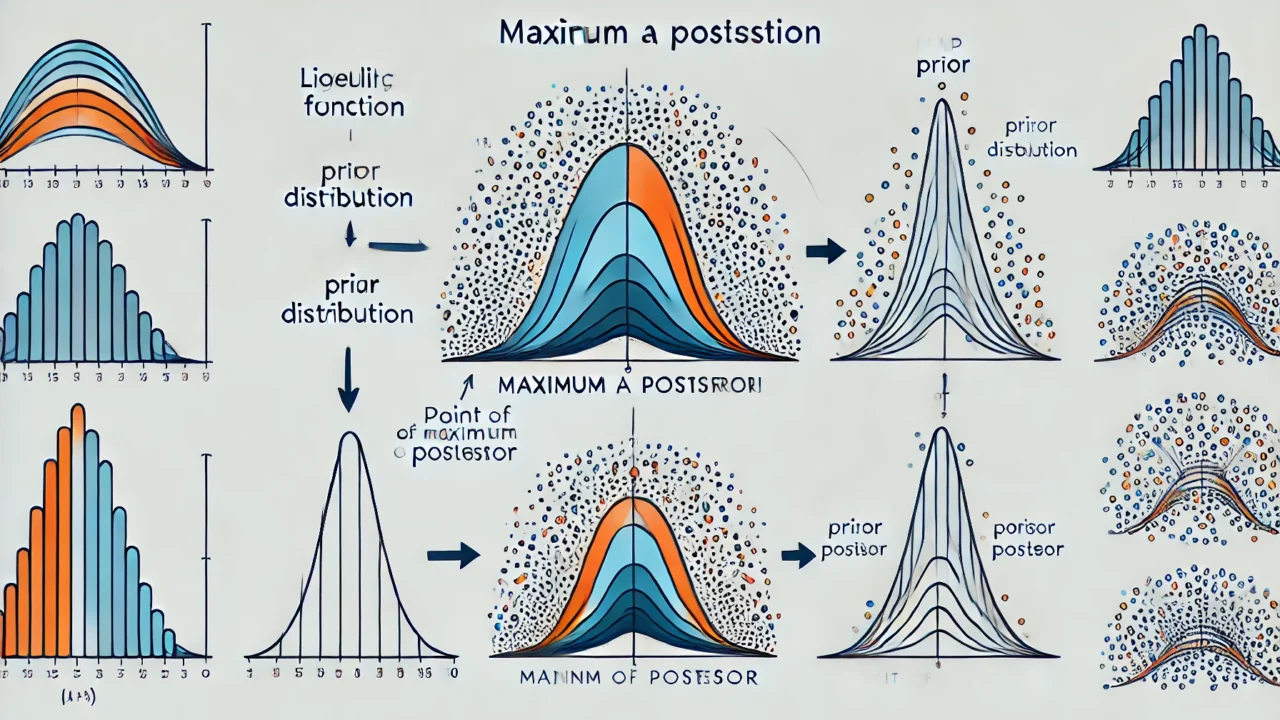
Maximum a Posteriori (MAP) estimation is a popular method in Bayesian statistics to estimate an unknown quantity.
MAP Estimation
MAP estimation aims to find the mode of the posterior distribution. Given a set of observed data \( \mathbf{X} = {x_1, x_2, \ldots, x_n} \) and a parameter \( \theta \) to be estimated, the MAP estimate is defined as:
$$ \hat{\theta}{\text{MAP}} = \arg\max{\theta} P(\theta \mid \mathbf{X}) $$
Using Bayes’ theorem, the posterior distribution \( P(\theta \mid \mathbf{X}) \) can be expressed as:
$$ P(\theta \mid \mathbf{X}) = \frac{P(\mathbf{X} \mid \theta) P(\theta)}{P(\mathbf{X})} $$
Since \( P(\mathbf{X}) \) is a constant with respect to \( \theta \), the MAP estimate simplifies to:
$$ \hat{\theta}{\text{MAP}} = \arg\max{\theta} P(\mathbf{X} \mid \theta) P(\theta) $$
Thus, we need to maximize the product of the likelihood \( P(\mathbf{X} \mid \theta) \) and the prior \( P(\theta) \).
Detailed Proof
Let’s consider the logarithm of the posterior distribution for computational convenience. The logarithm is a monotonic function, so the value of \( \theta \) that maximizes the posterior will also maximize the log-posterior:
$$\hat{\theta}{\text{MAP}} = \arg\max{\theta} \log P(\mathbf{X} \mid \theta) + \log P(\theta)$$
- Likelihood \( P(\mathbf{X} \mid \theta) \): The likelihood function is the probability of the observed data given the parameter \( \theta \).
$$ P(\mathbf{X} \mid \theta) = \prod_{i=1}^{n} P(x_i \mid \theta)
$$ Taking the logarithm, we get:
$$\log P(\mathbf{X} \mid \theta) = \sum_{i=1}^{n} \log P(x_i \mid \theta)
$$ - Prior \( P(\theta) \): The prior distribution reflects our beliefs about \( \theta \) before observing the data. Common choices for priors include uniform, Gaussian, or other distributions depending on the problem context.
- Posterior Maximization: Combining the log-likelihood and the log-prior, we have: $$ \hat{\theta}{\text{MAP}} = \arg\max{\theta} \left( \sum_{i=1}^{n} \log P(x_i \mid \theta) + \log P(\theta) \right)$$ This equation shows that the MAP estimate balances the fit of the model to the data (through the likelihood) with the prior belief about \( \theta \).
Example
Suppose we have a Gaussian likelihood and a Gaussian prior. The observed data \( x_1, x_2, \ldots, x_n \) are assumed to be normally distributed with mean \( \mu \) and known variance \( \sigma^2 \):
$$ P(x_i \mid \mu) = \frac{1}{\sqrt{2 \pi \sigma^2}} \exp \left( -\frac{(x_i – \mu)^2}{2 \sigma^2} \right) $$
If the prior distribution for \( \mu \) is also Gaussian with mean \( \mu_0 \) and variance \( \tau^2 \):
$$ P(\mu) = \frac{1}{\sqrt{2 \pi \tau^2}} \exp \left( -\frac{(\mu – \mu_0)^2}{2 \tau^2} \right) $$
The log-posterior is then:
$$ \log P(\mathbf{X} \mid \mu) + \log P(\mu) = -\frac{n}{2} \log(2 \pi \sigma^2) – \frac{1}{2 \sigma^2} \sum_{i=1}^{n} (x_i – \mu)^2 – \frac{1}{2} \log(2 \pi \tau^2) – \frac{1}{2 \tau^2} (\mu – \mu_0)^2 $$
Ignoring constant terms and simplifying, we get:
$$ \hat{\mu}{\text{MAP}} = \arg\max{\mu} \left( -\frac{1}{2 \sigma^2} \sum_{i=1}^{n} (x_i – \mu)^2 – \frac{1}{2 \tau^2} (\mu – \mu_0)^2 \right) $$
This can be solved by taking the derivative with respect to \( \mu \), setting it to zero, and solving for \( \mu \):
$$ \frac{\partial}{\partial \mu} \left( -\frac{1}{2 \sigma^2} \sum_{i=1}^{n} (x_i – \mu)^2 – \frac{1}{2 \tau^2} (\mu – \mu_0)^2 \right) = 0 $$
$$ \frac{1}{\sigma^2} \sum_{i=1}^{n} (x_i – \mu) + \frac{1}{\tau^2} (\mu – \mu_0) = 0 $$
$$ \mu \left( \frac{n}{\sigma^2} + \frac{1}{\tau^2} \right) = \frac{1}{\sigma^2} \sum_{i=1}^{n} x_i + \frac{\mu_0}{\tau^2} $$
$$ \hat{\mu}{\text{MAP}} = \frac{\frac{1}{\sigma^2} \sum{i=1}^{n} x_i + \frac{\mu_0}{\tau^2}}{\frac{n}{\sigma^2} + \frac{1}{\tau^2}} $$
This result shows that the MAP estimate is a weighted average of the sample mean and the prior mean, with weights inversely proportional to their variances.


