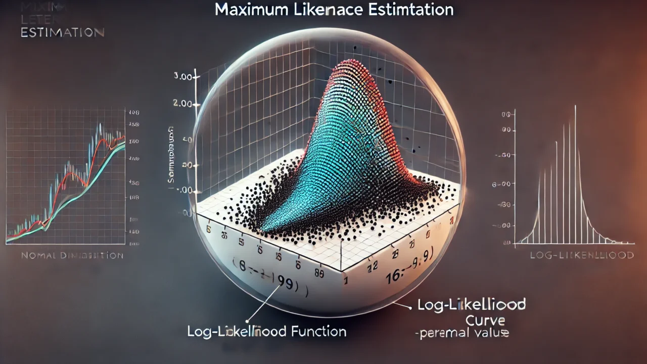
Maximum Likelihood Estimation (MLE) is a method used to estimate the parameters of a statistical model. The goal of MLE is to find the parameter values that maximize the likelihood function.
Likelihood Function
Suppose we have a set of observations \( \{x_1, x_2, \ldots, x_n\} \) that are independently and identically distributed (i.i.d) according to some probability distribution with parameter \( \theta \). The likelihood function \( L(\theta) \) is defined as the joint probability (or probability density) of the observed data as a function of \( \theta \):
$$ L(\theta) = P(x_1, x_2, \ldots, x_n \mid \theta) = \prod_{i=1}^n P(x_i \mid \theta) $$
Log-Likelihood Function
In practice, it is often easier to work with the natural logarithm of the likelihood function, known as the log-likelihood function:
$$ \ell(\theta) = \log L(\theta) = \log \left( \prod_{i=1}^n P(x_i \mid \theta) \right) = \sum_{i=1}^n \log P(x_i \mid \theta) $$
Maximum Likelihood Estimate
The maximum likelihood estimate (MLE) of the parameter \( \theta \) is the value that maximizes the log-likelihood function:
$$ \hat{\theta} = \arg \max_\theta \ell(\theta) $$
Example: Normal Distribution
Consider a set of i.i.d observations \( \{x_1, x_2, \ldots, x_n\} \) from a normal distribution with unknown mean \( \mu \) and known variance \( \sigma^2 \). The probability density function is:
$$ f(x \mid \mu) = \frac{1}{\sqrt{2 \pi \sigma^2}} \exp \left( -\frac{(x – \mu)^2}{2\sigma^2} \right) $$
The log-likelihood function is:
$$ \ell(\mu) = \sum_{i=1}^n \log f(x_i \mid \mu) = -\frac{n}{2} \log (2 \pi \sigma^2) – \frac{1}{2\sigma^2} \sum_{i=1}^n (x_i – \mu)^2 $$
To find the MLE, we take the derivative of \( \ell(\mu) \) with respect to \( \mu \) and set it to zero:
$$ \frac{d\ell(\mu)}{d\mu} = \frac{1}{\sigma^2} \sum_{i=1}^n (x_i – \mu) = 0 $$
Solving for \( \mu \), we get the MLE:
$$ \hat{\mu} = \frac{1}{n} \sum_{i=1}^n x_i $$
Properties of MLE
Under certain regularity conditions, the MLE has several desirable properties:
Consistency:
The MLE converges in probability to the true parameter value as the sample size increases.
Asymptotic Normality:
The distribution of the MLE approaches a normal distribution as the sample size increases.
Efficiency:
The MLE achieves the Cramér-Rao lower bound, meaning it has the lowest possible variance among unbiased estimators.


